Formulas and functions
You can add functions to the spreadsheet in order to perform calculations, for example. Different formulas are available to you, depending on whether you are editing a model of the Spreadsheet type, a results table of a query, or an ad hoc analysis.
Logical AND operation.
AND requires at least one argument. You can use single arguments and/or scope arguments.
Value 1 | Value 2 | AND |
Example 39. FALSE | Example 40. FALSE | Example 41. FALSE |
Example 42. FALSE | Example 43. TRUE | Example 44. FALSE |
Example 45. TRUE | Example 46. FALSE | Example 47. FALSE |
Example 48. TRUE | Example 49. TRUE | Example 50. TRUE |
=AND (TRUE;TRUE) returns the following:

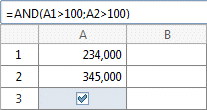
=AND(A1>100;A2>100) returns TRUE.
Indicates an attribute.
ARIS_ATTRIBUTE requires an API name of an attribute as input and displays the name of the attribute in the cell.
The following formula outputs the name of the ARIS attribute Name. Required input is the API name.
=ARIS_ATTRIBUTE("AT_NAME")

For result tables for queries or ad-hoc analyses, replace ARIS with QUERY or ANALYSIS in the formula.
Outputs an attribute value.
ARIS_ATTRIBUTE_VALUE requires an ARIS item and an attribute as input. You can only use single arguments.
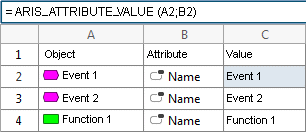
For a model of type Spreadsheet, the following formula outputs the attribute value of the ARIS item that is displayed in cell A2 and whose Name attribute is specified in cell B2.
=ARIS_ATTRIBUTE_VALUE(A2;B2)
=ARIS_ATTRIBUTE_VALUE(ARIS_ITEM("GUID");ARIS_ATTRIBUTE("API name of the attribute"))
For result tables for queries or ad-hoc analyses, replace ARIS with QUERY or ANALYSIS in the formula.
Indicates an ARIS item.
An item is an:
ARIS model
ARIS object
ARIS connection
ARIS_ITEM requires a GUID with quotation marks as an argument. The input is entered in the following form:
=ARIS_ITEM("GUID")
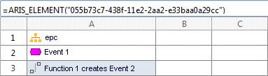
For a model of type Spreadsheet, the formula outputs the name of the ARIS item and the associated symbol.
The cell of the connection is selected. The formula outputs the name and the connection symbol.
=ARIS_ITEM("ff14b3a1-438e-11e2-2aa2-e33baa0a29cc")
For result tables for queries or ad-hoc analyses, replace ARIS with QUERY or ANALYSIS in the formula.
Returns the API name of an ARIS item.
An item is an:
ARIS model
ARIS object
ARIS connection
ARIS_ITEM_API_NAME requires an ARIS item as an argument.
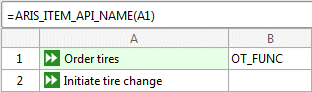
In this example, the API name of the item in cell A1 is output in cell B1.
=ARIS_ITEM_API_NAME(A1)
For result tables for queries or ad-hoc analyses, replace ARIS with QUERY or ANALYSIS in the formula.
Returns the name of the default symbol for an ARIS object.
ARIS_ITEM_DEF_SYMBOL requires an ARIS item as an argument.
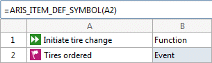
In this example, the default symbol names for the items of cell A1 and A2 are displayed in cell B1 and B2.
=ARIS_ITEM_DEF_SYMBOL(A1)
=ARIS_ITEM_DEF_SYMBOL(A2)
For result tables for queries or ad-hoc analyses, replace ARIS with QUERY or ANALYSIS in the formula.
Returns the GUID of the ARIS item.
ARIS_ITEM_GUID requires an ARIS item as input. This can be a cell containing an ARIS item, or the result of a calculation that returns an ARIS item.
For a model of type Spreadsheet, the following formula returns the GUID of the ARIS item that appears in cell A1.
=ARIS_ITEM_GUID(A1)

For result tables for queries or ad-hoc analyses, replace ARIS with QUERY or ANALYSIS in the formula.
Returns the path to an ARIS item.
ARIS_ITEM_PATH requires an ARIS item as input.
For a model of type Spreadsheet, the following formula returns the path to the ARIS item of cell A1.
=ARIS_ITEM_PATH(A1)

For result tables for queries or ad-hoc analyses, replace ARIS with QUERY or ANALYSIS in the formula.
Returns the type of an ARIS item.
ARIS_ITEM_TYPE requires an ARIS item as input.
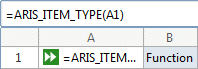
For a model of type Spreadsheet, the following formula returns the type of an ARIS item of cell A1.
=ARIS_ITEM_TYPE(A1)
For result tables for queries or ad-hoc analyses, replace ARIS with QUERY or ANALYSIS in the formula.
Returns the type number of an ARIS item.
ARIS_ITEM_TYPE_NUM requires an ARIS item as input.
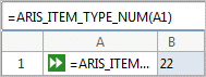
For a model of Spreadsheet type, the following formula returns the type number of the ARIS item of cell A1.
ARIS_ITEM_TYPE_NUM=(A1)
For result tables for queries or ad-hoc analyses, replace ARIS with QUERY or ANALYSIS in the formula.
Indicates whether or not an ARIS item is locked by a user. The user is displayed in the Spreadsheet model.
An item is an:
ARIS model
ARIS object
ARIS_LOCKED_BY_USER requires a cell reference of the models or objects as an argument. The input is entered in the following form:
=ARIS_LOCKED_BY_USER(cell reference)
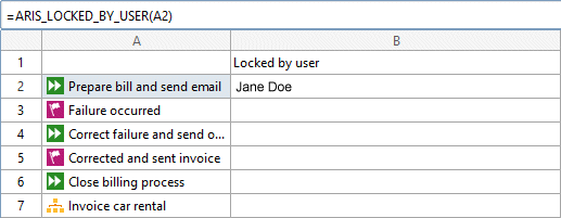
For a model of type Spreadsheet, the formula outputs the name of the user who has locked models or objects. The cell of the object is selected.
=ARIS_LOCKED_BY_USER(A2)
Specifies the attribute value of an object.
ARIS_WRITE_ATTRIBUTE_VALUE requires as input an ARIS item, an attribute, and the value that the attribute is to receive. You can only use single arguments
For a model of type Spreadsheet, the following formula sets the attribute value of the ARIS item that is displayed in cell A1 and whose attribute is specified in cell B1 to acceptable.
=ARIS_WRITE_ATTRIBUTE_VALUE(A1;B1;"acceptable")
For result tables for queries or ad-hoc analyses, replace ARIS with QUERY or ANALYSIS in the formula.
Returns the average.
AVERAGE requires at least one argument. You can use single arguments and/or scope arguments.
AVERAGE(A1:A5) returns the average of the values saved in the cells A1 to A5.
Returns a value based on an index.
Indexing means the position of an item in a list. If for example, you have a list with the values 1,3,5,7,13, the item at position three has the value five.
CHOOSE requires at least two arguments. The first argument represents the index of the value that the corresponding item is selected from.
Input: CHOOSE(Position of the item, Item1..Item2)
CHOOSE(1;2;4;6;8;19) returns 2
CHOOSE(3;2;4;6;8;19) returns 6
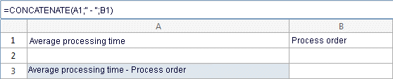
Concatenates strings that are separated by a semicolon.
Calculates the number of arguments. You can use single arguments and/or scope arguments.
=COUNT(A1;12;5) returns 3, because three arguments are transferred.
=COUNT(A1:A3;"Text") returns 4, because four arguments are transferred.
=COUNT(A1:A5) returns 5.
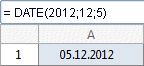
Converts three numeric arguments into a date.
The input of the arguments is made in the following form: =DATE(Year;Month;Day), also =DATE(YYYY;MM;DD)
=DATE(2012;12;5) returns the date 5.12.2012.
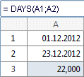
Returns the number of days between two dates.
The date cannot be entered directly as an argument, but must be present in cells or be calculated by a formula that returns a value of the Date type. Two arguments are required.
The input of the arguments is made in the following form: =DAYS(Date;Date).
=DAYS(A1;A2) returns 22 days.
Checks a condition and returns a value depending on the result.
IF requires three arguments. The input is entered in the following form:
IF(Condition;Condition met;Condition not met).
When you enter =IF(A1>A2;1;0) you receive TRUE.
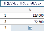
When you enter =IF(A1>A2;TRUE;FALSE) you receive the following:
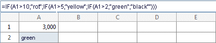
When you enter =IF(A1>10;"red";IF(A1>5;"yellow";IF(A1>2;"green";"black"))) you receive the following:
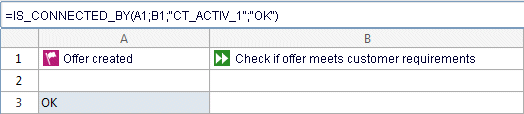
Returns the specified string if source object and target object are connected via the respective connection type
IS_CONNECTED_BY requires as input at least one ARIS source object, an ARIS target object, the API name of the connection type, and the string to be displayed if this relationship exists at the definition level. You can only use single arguments
The following formula outputs the string OK, if the source object is connected to the target object via the connection activates with the API name CT_ACTIV_1.
=IS_CONNECTED_BY(A1;B1;"CT_ACTIV_1";"OK")
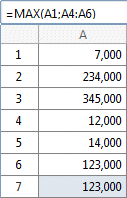
Returns the maximum value in a list of arguments. MAX requires at least one argument. You can use single arguments and/or scope arguments.
=MAX(A1;A4:A6) returns 123.
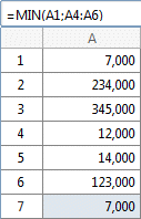
Returns the minimum value in a list of arguments. MIN requires at least one argument. You can use single arguments and/or scope arguments.
=MIN(A1;A4:A6) returns 7.
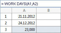
Returns the work days between two dates.
NETWORKDAYS requires two arguments and returns the work days assuming that Saturday and Sunday are days off.
Logical inversion.
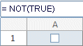
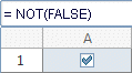
NOT requires the argument True or False.
NOT(TRUE) or NOT(1) returns FALSE and NOT(FALSE) or NOT(0) returns TRUE.
NOT(TRUE)
NOT(FALSE)
Returns the current time.
NOW does not require any arguments.
The input is entered in the following form:
=NOW()
The NOW() function refreshes the time each time a calculation is carried out in the spreadsheet.
Logical OR operation.
OR requires at least one argument.
Value 1 | Value 2 | OR |
|---|---|---|
Example 75. FALSE | Example 76. FALSE | Example 77. FALSE |
Example 78. FALSE | Example 79. TRUE | Example 80. TRUE |
Example 81. TRUE | Example 82. FALSE | Example 83. TRUE |
Example 84. TRUE | Example 85. TRUE | Example 86. TRUE |
Returns the square root of a number.
SQRT requires an argument.
=SQRT(4) returns two.
Normalizes to one hundred percent.
STANDARDIZE requires three arguments and normalizes a value that lies between a minimum and maximum value. The calculation is made as follows:
The first argument represents the value, the difference of the two following ones the range that is normalized to one hundred percent.
(Value - Minimum) / (Maximum - Minimum)
STANDARDIZE is mainly used for a cell with conditional formatting to highlight the maximum value reached by not coloring the cell at all, coloring it partially, or coloring it completely.
STANDARDIZE(2;0;10) equates to (2-0)/(10-0) and results in 0,2
STANDARDIZE(7;3;10) equates to (7-3)/(10-3) and results in 0.571
Returns the sum of argument values.
SUM requires at least one argument.
=SUM(2;3) returns five.
Checks a condition and reacts according to the defined conditions.
SWITCH requires at least three arguments: a condition and a value that is displayed when the condition is met, and a default value that is displayed when none of the conditions listed is met.
It is also possible to link conditions with the IF formula. This however, would require a longer expression.
=SWITCH(A1>10;"red";A1>5;"yellow";A1>2;"green";"black")
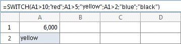
In comparison, the expression when IF is used:
=IF(A1>10;"red";IF(A1>5;"yellow";IF(A1>2;"green";"black")))
Returns a time.
TIME requires three arguments.
The input is entered in the following form:
=TIME(Hour;Minute;Second)
=TIME(2;23;59) returns 2:23:59
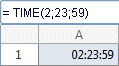
The input of =TIME(25;23;59) returns 1:23:59.
The input of =TIME(2;23;61) returns 2:24:01.
Returns the current date.
TODAY does not require any arguments.
The input is entered in the following form:
=TODAY()
The TODAY() function refreshes the date each time a calculation is carried out in the spreadsheet.
Logical XOR operation.
XOR requires at least one argument.
A1 | A2 | XOR |
|---|---|---|
Example 92. FALSE | Example 93. FALSE | Example 94. FALSE |
Example 95. FALSE | Example 96. TRUE | Example 97. TRUE |
Example 98. TRUE | Example 99. FALSE | Example 100. TRUE |
Example 101. TRUE | Example 102. TRUE | Example 103. FALSE |